Neural habituation enhances novelty detection: an EEG study of rapidly presented words
Published on the peer-reviewed journal Computational Brain & Behavior.
Pre-print available on bioRxiv.
This page summarizes the two computational models used in the project:
- The machine learning SVM model that predicts trial-by-trial subject behavior based on neural data;
- The neural network model that simulates temporal parsing in vision and predicts average subject behavior and average neural activity.
The overarching goal of this research was to study how the visual system parses information over time. More specifically, the research tested a theory called ‘neural habituation’. According to this theory, persistent neural activity consumes synaptic resources (neurotransmitters). This resource depletion in the active neuronal population causes the neural response to repeated stimuli to be dampened, thus allowing the visual system to more easily perceive novel stimuli. In summary, the theory states that resource depletion, which is typically seen as a setback, can be beneficial, as it enhances novelty detection.
For better understanding of the models, a basic explanation of the experimental task performed by the subjects is included below. For further details, please refer to the section “Experimental design and behavioral data analysis” within “Material and Methods” in the paper.
Experimental task
Subjects performed a word identification task, illustrated in the figure below:
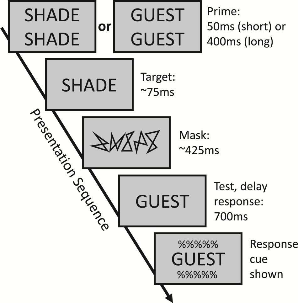
Each trial began with the presentation of a doubled-up “prime” word. The goal of this word was to change how subsequent words in the trial are processed by the visual system. The prime word could be presented for a “short” duration of 50ms (which should generate less resource depletion, and thus less neural habituation), or for a “long” duration of 400ms (more resource depletion, and more neural habituation.
Immediately after presentation of the prime, a “target” word was shown. It was flashed briefly for around 75ms. Subjects were instructed to pay attention and identify this target word.
After target word presentation, a “perceptual mask” consisting of randomly-generated lines was shown. The goal of the mask was to reduce visibility of the target word, making the task more difficult.
Finally, a test display consisting of a single “response” word was presented. Subjects had to decide whether this word was the “same” or “different” from the target word. In the figure above, the correct answer would be “different”. Subjects indicated their choice by pressing a button once a response cue was displayed.
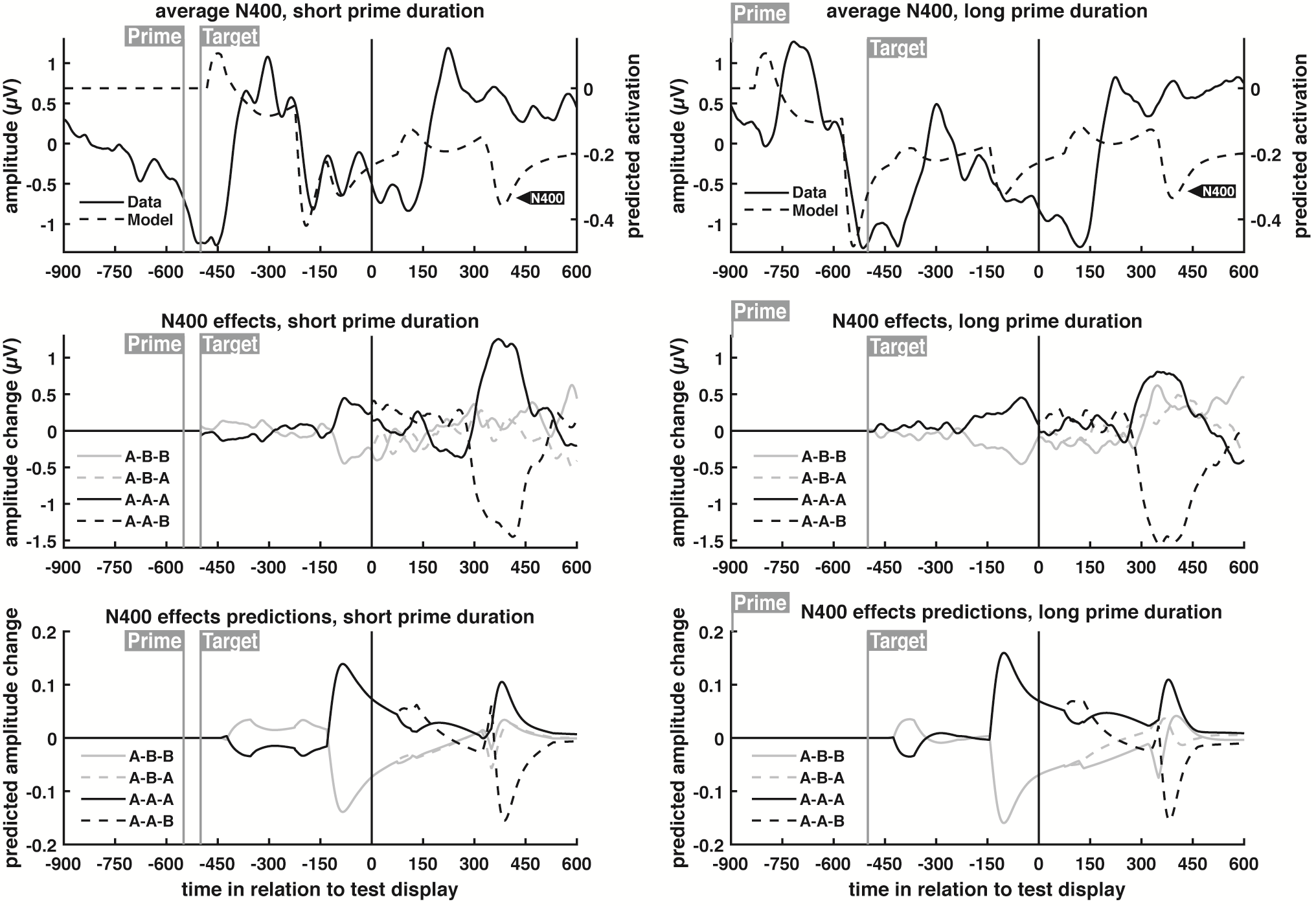
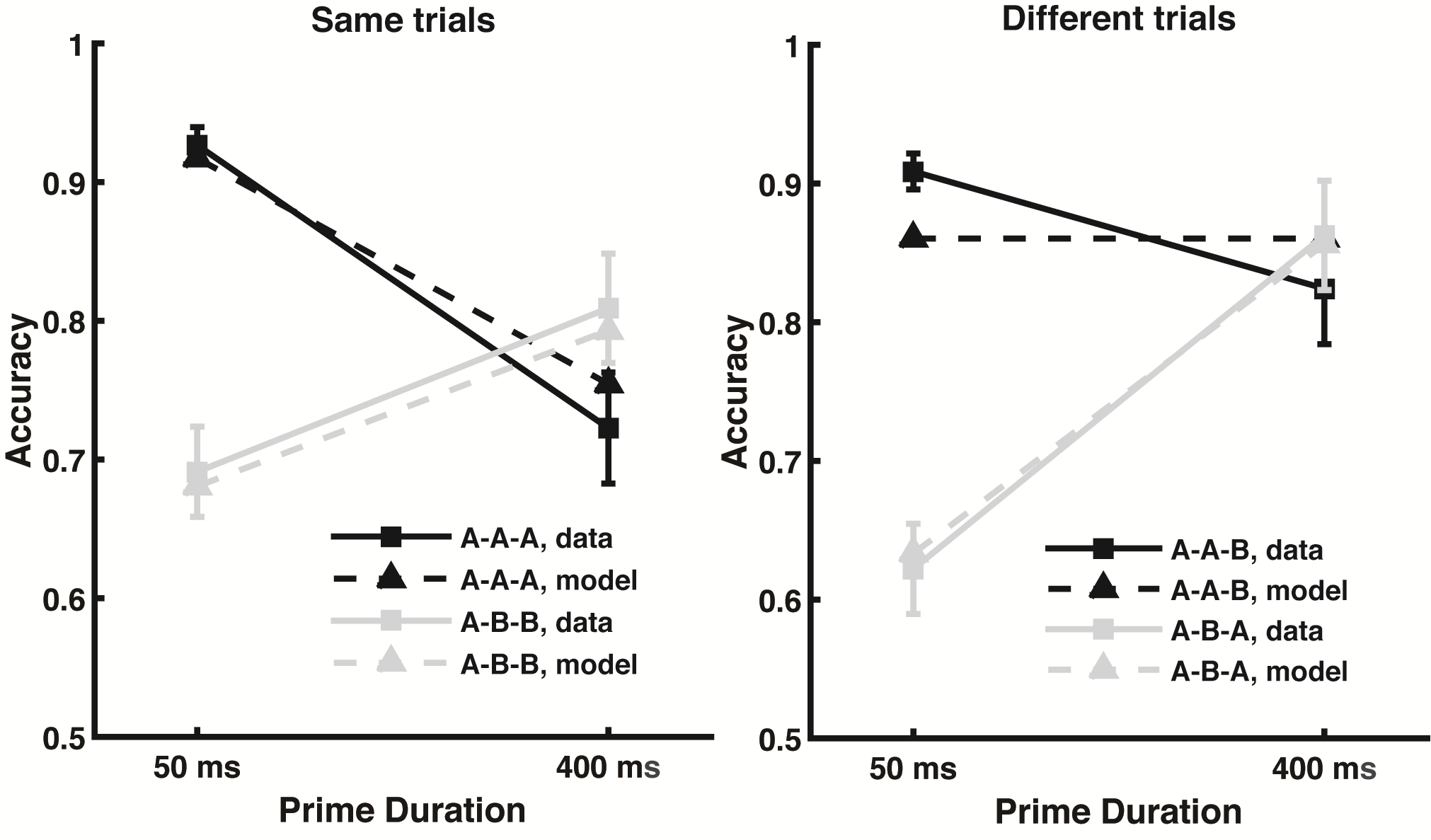
Each trial used a unique set of words, and each subjected responded to a total of 640 trials. There were 8 experimental conditions total, and subjects performed 60 trials of each condition. These conditions were a product of three factors, each with two levels: prime duration (long or short), whether the response word matched the prime word (primed or unprimed), and what was the correct answer for the trial (same or different). In labeling these conditions, the letters A or B are used to refer to each word in the sequence of events (each trial required no more than two unique words), across the prime, target, and response word presentations. Thus, the same-primed condition is A-A-A (the same word for all three presentations), the same-unprimed condition is A-B-B, the different-primed condition is A-B-A, and the different-unprimed condition is A-A-B.
Machine learning SVM model (code)
The goal of the SVM (support vector machine) model was to predict subject choice (whether they pressed the button that corresponded to “same” or “different”).
The model was trained on neural EEG (electroencephalogram) data collected during the 700ms following response word presentation, during which subjects deliberated which button to press (they were told to delay any button presses to the moment the response cue was shown). These 700ms of neural data were split into 14 windows of 50ms each; then, each of these 50ms of data were averaged into a single value. This was done independently for each of the 64 EEG sensors, resulting in a 64 (sensors) by 14 (time windows) data matrix for each experimental trial. The data from each trial was then normalized via z-scoring.
Prior to model training, data was set aside for validation. To parse out variability from random sampling, training and validation was conducted 1000 times. Each time, 40 trials for each subject were set aside for validation (5 randomly selected trials from each of the 8 conditions), and the model was trained on all remaining trials (aggregated from all subjects and conditions). Then, the model was validated on the held-out trials. Validation was done three ways: all subjects and conditions to obtain global performance, then on each subject at a time, then on each condition at a time. Model performance was saved, then everything was wiped clean and a new model was trained and validated. Finally, performance from the 1000 models were averaged.
The model predicted subject choice with 66.34% accuracy, a strikingly high value given the large amount of noise present in individual EEG trials. The classifier was above chance for all subjects; the lowest classification performance when validating on an individual subject was 56.38%, showing that the classifier succeeded in finding the neural signals shared between each individual’s unique brain anatomy. Therefore, the next step was to identify the temporal profile of the shared neural signals driving the model’s predictions.
To that end, the model was trained and validated on each time window separately. The validation accuracy of each time window is shown below in (a), along with the model weights scalp maps of three highlighted time windows (b), and equivalent average neural data for the same windows (c).
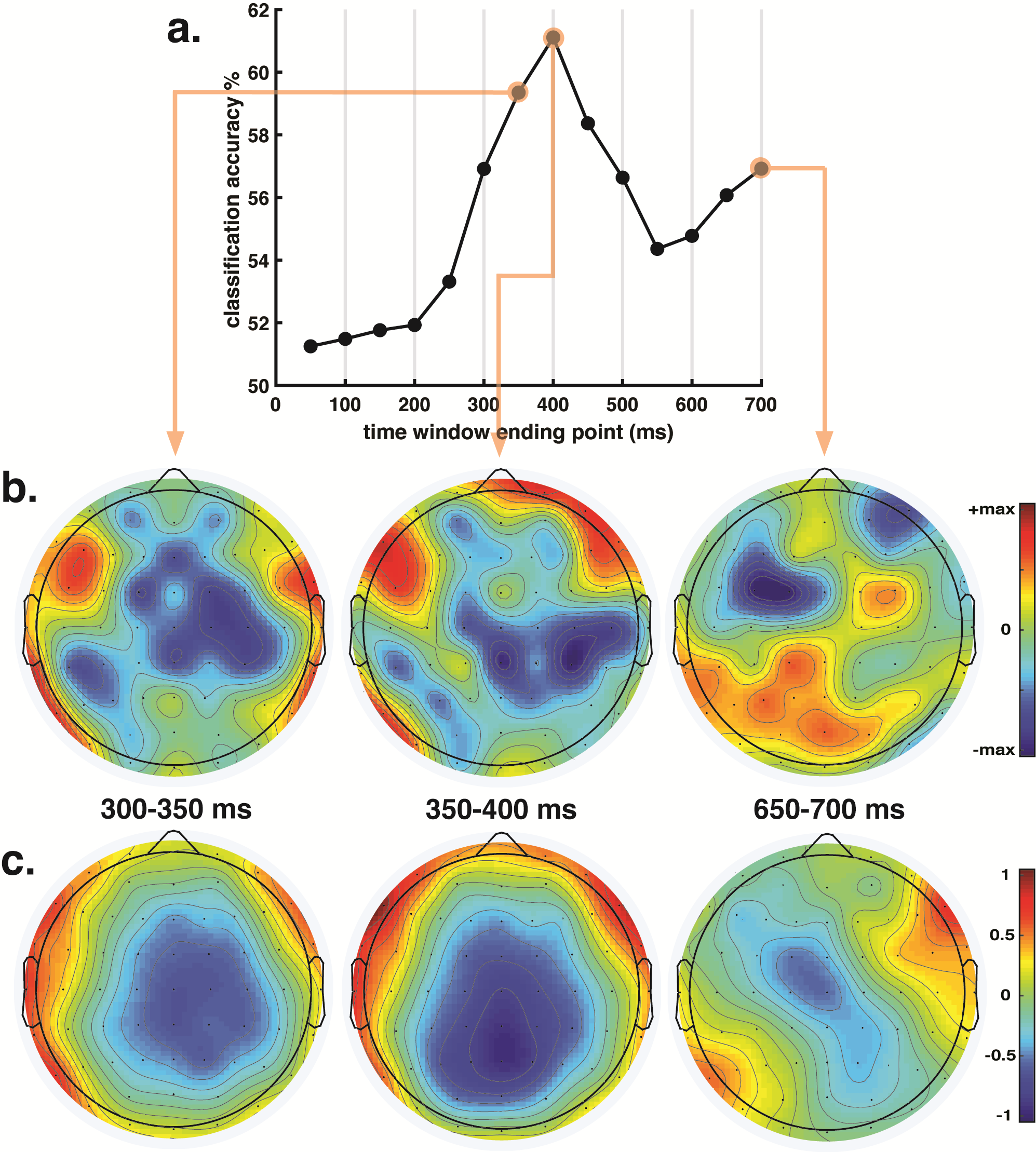
As seen in the figure, for the time windows immediately following response word presentation, accuracy is low and close to chance. This would be expected, considering the brain has not had enough time to process the word. Starting at the 200-250ms window, accuracy quickly rises, peaking at the 350-400ms window. Then, accuracy decreases, only to rise slightly shortly before response cue presentation.
The moderate increase in accuracy shortly before response cue presentation is attributed to movement planning (the weights scalp map in (b) and the neural data in (c) both display asymmetries between the two brain hemispheres that highlight this). But the result of interest is the accuracy peak at the 350-400 time window. The high predictive power of this individual window coincides with a well-known neural signal called the N400: a negative-voltage brain potential that typically peaks around 400ms following display of a word considered to be unexpected by readers (the N400 can be clearly seen in part “c” of the figure). However, the N400 potential can happen in several different contexts, and the scientific literature has struggled to formulate a comprehensive theory of its neural basis. The results of this SVM classifier, showing that the 350-400ms time window is predictive of behavior in a novelty detection task (i.e. is this new/different or old/same?), sheds new light in the neural basis of the N400 potential, and has important implications for the understanding of visual and linguistic processing.
Neural network model (code)
To test directly test the theory of neural habituation, an artificial neural network model that simulates temporal parsing was created, and resource depletion was implemented in the model through a series of mathematical equations. The model, therefore, simulates what is believed to be happening in the brain, and outputs behavior predictions (accuracy across different conditions in the experimental task) and neural activity predictions (the average shape of EEG waveforms displayed by subjects undergoing the experiment). If the theory underlying the model actually represents what is happening within the brain, the model’s predictions will be very similar to the observed data collected from participants.
The model structured is displayed in the schematic below. It is organized in four layers, equivalent to four functional areas of the brain that represent progressively more complex stimuli. Each layer is formed by nodes, and each node represents large groups of neurons that respond to the same stimulus. As shown in the figure, these nodes connect to each other via excitatory or inhibitory connections.
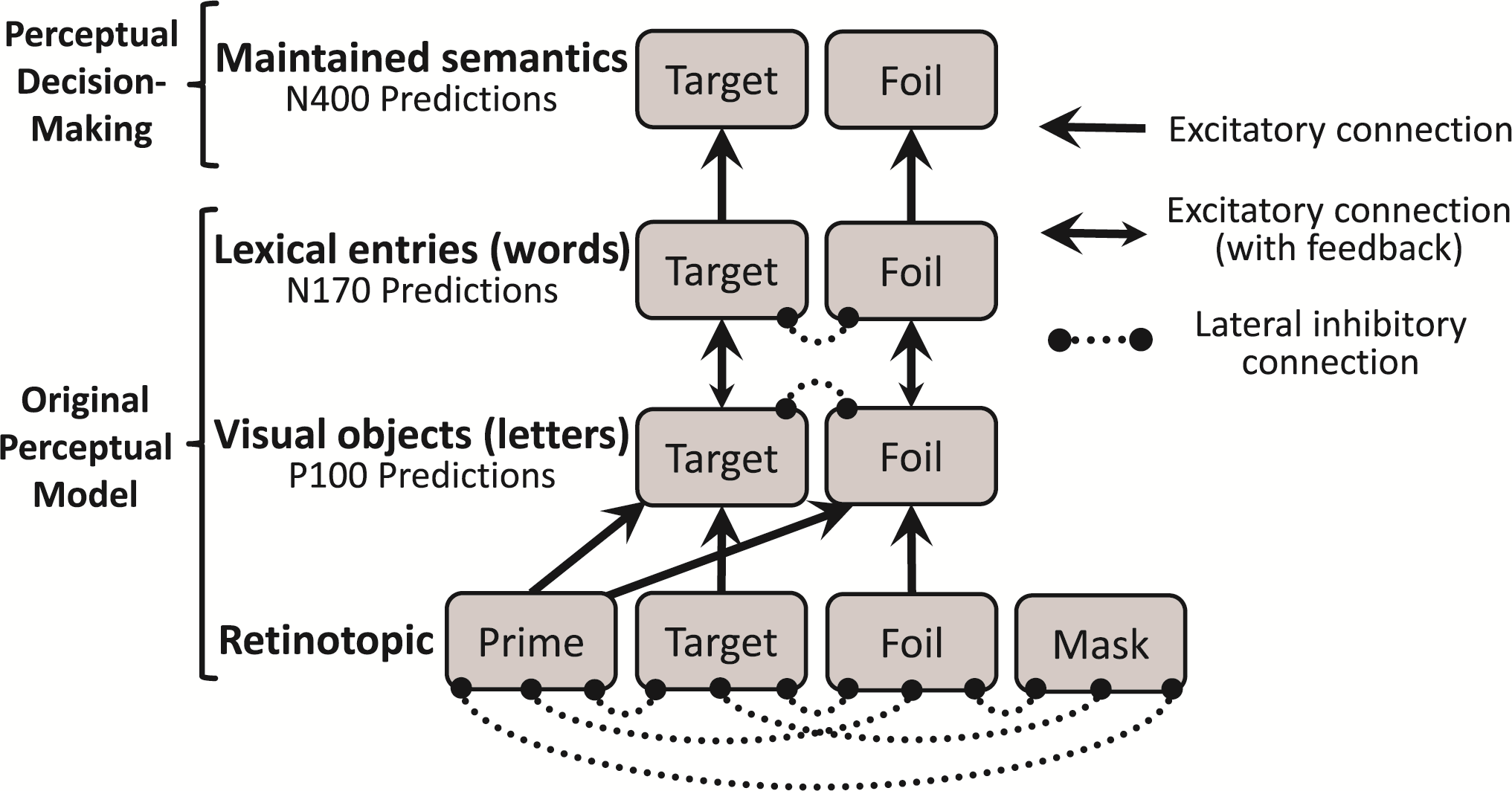
The first (bottom) layer is the retinotopic layer; it represents line segments within different positions of the visual field. The second layer represents simple visual objects irrespective of position (in the case of the present task, it represents individual letters). The third layer represents more complex objects: lexical entries (words). These three layers together form the perceptual basis of the model (i.e. what is being seen right now). In order for the model to make same/different decisions, it needs a fourth layer: named maintained semantics, it acts as the model’s working memory, allowing it to retain the identity of previously seen words for short periods of time.
To assess whether the response word is “same” or “different” than the target word, the key determinant is how easy it is to update working memory to also include the meaning of the response word. If the response word is already in working memory, it will have a high residual activity in the maintained semantics layer, and it will therefore be easy to update working memory to include that word’s identity. However, if that word was not seen previously in the trial, there will be little or no residual activation for that word, making it more difficult to update working memory with it, and suggesting that the correct answer is “different”. As seen in the figure below, the model’s predictions were very close to the observed data.
Predictions for EEG neural activity are obtained by summing the output of all nodes within a layer (the EEG method has low spatial resolution, and thus cannot separate the neural signal of each individual word). The model is capable of predicting three different neural potentials: the P100 (a positive-voltage brain potential that typically occurs around 100ms after presentation of a visual stimulus, and reflects the processing of simple visual objects, such as the letters in a word), the N170 (a negative-voltage brain potential that typically occurs around 170ms after presentation of a visual stimulus, and reflects the processing of more complex visual objects, such as full words), and the N400 (a negative-voltage brain potential that typically occurs around 400ms after presentation of visual stimulus, and reflects the processing of unexpected stimuli).
Predictions for the N400 neural potential are shown below (for P100/N170 predictions, please refer to the section “ERP results” in the paper). The neural network model used parameters that best fit the behavioral data, and it was never fit to the neural data. Therefore, the model’s ability to predict the neural data is particularly striking, especially when it comes to the condition effects (second and third rows). Taken together, this supports the theory of neural habituation.